Mathematical AnalysisIntegral Calculus |
What is the graphic representation of the approximation of an area under a curve using integration? |
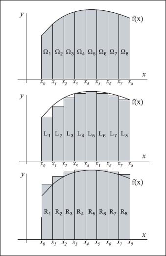
It’s easier to see the approximate area under a curve using integration by means of graphs—it all has to do with rectangles. The idea is to extend lines from the ends of the curve (here, f(x)) to the x-axis (or y-axis, depending on the curve); we’ll call the total area under the curve Ω, then divide the entire area under the curve into equal-width sections (x1, x2, x3, and so on) that are equal to parts of Ω (the subregions Ω1 Ω2, and so on). The next step is to figure out the area of a rectangle if each section was “cut off” below the curve and then above the curve. This creates rectangles defined by left- and right-end points. From the left- and right-sums, and a few more calculations, we can approximate the area of Ω. This can be seen graphically on the accompanying charts.

To calculate the area beneath a curve (top), you can first divide the area into equal parts with rectangles both beneath (middle) and above (bottom) the curve. Adjusting the width of the curves will result in an estimate that closely approximates the actual area.
